Data analyzes I - basics in data handling

Edited by Yury Markov (he/him) Peer Herholz (he/him)
Habilitation candidate - Fiebach Lab, Neurocognitive Psychology at Goethe-University Frankfurt
Research affiliate - NeuroDataScience lab at MNI/McGill
Member - BIDS, ReproNim, Brainhack, Neuromod, OHBM SEA-SIG, UNIQUE

  @peerherholz

Before we get started …

• most of what you’ll see within this lecture was prepared by Ross Markello, Michael Notter and Peer Herholz and further adapted for this course by Peer Herholz

• based on Tal Yarkoni’s “Introduction to Python” lecture at Neurohackademy 2019

• based on 10 minutes to pandas

Objectives 📍

• learn basic and efficient usage of python for data analyzes & visualization

  • working with data:

    • reading, working, writing

    • preprocessing, filtering, wrangling

  • visualizing data:

    • basic plots

    • advanced & fancy stuff

Why do data science in Python?

• all the general benefits of the Python language (open source, fast, etc.)

  • Specifically, it’s a widely used/very flexible, high-level, general-purpose, dynamic programming language

• the Python ecosystem contains tens of thousands of packages, several are very widely used in data science applications:

  • Jupyter: interactive notebooks

  • Numpy: numerical computing in Python

  • pandas: data structures for Python

  • pingouin: statistics in Python

  • statsmodels: statistics in Python

  • seaborn: data visualization in Python

  • plotly: interactive data visualization in Python

  • Scipy: scientific Python tools

  • Matplotlib: plotting in Python

  • scikit-learn: machine learning in Python

• even more: Python has very good (often best-in-class) external packages for almost everything

• Particularly important for data science, which draws on a very broad toolkit

• Package management is easy (conda, pip)

• Examples for further important/central python data science packages :

  • Web development: flask, Django

  • Database ORMs: SQLAlchemy, Django ORM (w/ adapters for all major DBs)

  • Scraping/parsing text/markup: beautifulsoup, scrapy

  • Natural language processing (NLP): nltk, gensim, textblob

  • Numerical computation and data analysis: numpy, scipy, pandas, xarray

  • Machine learning: scikit-learn, Tensorflow, keras

  • Image processing: pillow, scikit-image, OpenCV

  • Plotting: matplotlib, seaborn, altair, ggplot, Bokeh

  • GUI development: pyQT, wxPython

  • Testing: py.test

Widely-used

• Python is the fastest-growing major programming language

• Top 3 overall (with JavaScript, Java)

What we will do in this section of the course is a short introduction to Python for data analyses including basic data operations like file reading and wrangling, as well as statistics and data visualization. The goal is to showcase crucial tools/resources and their underlying working principles to allow further more in-depth exploration and direct application.

It is divided into the following chapters:

• Getting ready

• Basic data operations

  • Reading data

  • Exploring data

• Basic data visualization

  • Underlying principles

  • “standard” plots

  • Going further with advanced plots

• Statistics in python

  • Descriptive analyses

  • Inferential analyses

• Interactive data visualization

Here’s what we will focus on in the first block:

• Getting ready

• Basic data operations

  • Reading data

  • Exploring data

  • Data wrangling

Getting ready

What’s the first thing we have to check/evaluate before we start working with data, no matter if in Python or any other software? That’s right: getting everything ready!

This includes outlining the core workflow and respective steps. Quite often, this notebook and its content included, this entails the following:

1. What kind of data do I have and where is it?

2. What is the goal of the data analyses?

3. How will the respective steps be implemented?

So let’s check these aspects out in slightly more detail.

Lets Download our dataset first: link. This dataset is based on Demo Stroop experiment from Psychopy

What kind of data do I have and where is it

The first crucial step is to get a brief idea of the kind of data we have, where it is, etc. to outline the subsequent parts of the workflow (python modules to use, analyses to conduct, etc.). At this point it’s important to note that Python and its modules work tremendously well for basically all kinds of data out there, no matter if behavior, neuroimaging, etc. . To keep things rather simple, we will use a behavioral dataset that contains ratings and demographic information from a group of university students (ah, the classics…).

Knowing that all data files are located in a folder called data_experiment on our desktop, we will use the os module to change our current working directory to our desktop to make things easier:

from os import chdir

chdir('C:/Users/ika_m/OneDrive - Johann Wolfgang Goethe Universität/Documents/test_data')

Now we can actually already start using Python to explore things further. For example, we can use the glob module to check what files are in this directory and obtain a respective list:

from glob import glob

data_files = glob('*.csv')

As you can see, we provide a path as input to the function and end with an *.csv which means that we would like to gather all files that are in this directory that end with .csv. If you already know more about your data, you could also use other expressions and patterns to restrain the file list to files with a certain name or extension.

So let’s see what we got. Remember, the function should output a list of all files in the specified directory.

data_files

['AG_01_02_stroop_2025-01-23_13h12.02.354.csv',
 'BF_31_01_stroop_2025-01-23_12h25.25.690.csv',
 'BF_31_02_stroop_2025-01-23_13h12.43.710.csv',
 'FB_09_02_stroop_2025-01-23_13h12.14.223.csv',
 'FB_09_03_stroop_2025-01-23_13h30.49.889.csv',
 'FK_24_01_stroop_2025-01-23_12h36.23.128.csv',
 'JB_22_01_stroop_2025-01-23_12h29.58.313.csv',
 'JB_22_02_stroop_2025-01-23_13h13.20.521.csv',
 'JB_22_03_stroop_2025-01-23_13h32.52.317.csv',
 'XY_16_03_stroop_2025-01-23_13h31.18.706.csv']

Coolio, that worked. We get a list indicating all files as items in the form of strings. We also see that we get the relative paths and that our files are in .csv format. Having everything in a list, we can make use of this great python data type and e.g. check how many files we have, as well as if we have a file for every participant (should be 10).

print(len(data_files))

if len(data_files)==10:
    print('The number of data files matches the number of participants.')
elif len(data_files) > 10:
    print('There are %s more data files than participants.' %str(int(len(data_files)-19)))
elif len(data_files) < 10:
    print('There are %s data files missing.' %str(19-len(data_files)))

10
The number of data files matches the number of participants.

We also saw that some files contain a ' ', i.e. space, and knowing that this can cause major problems when coding analyzes, we will use python again to rename them. Specifically, we will use the rename function of the os module. It expects the old file name and the new file name as positional arguments, i.e. os.rename(old_file_name, new_file_name). While renaming, we follow “best practices” and will replace the space with an _. In order to avoid doing this manually for all files, we will just use a combination of a for loop and an if statement:

from os import rename

for file in data_files:
    if ' ' in file:
        rename(file, file.replace(' ', "_"))

data_files = glob('*.csv')

data_files

['AG_01_02_stroop_2025-01-23_13h12.02.354.csv',
 'BF_31_01_stroop_2025-01-23_12h25.25.690.csv',
 'BF_31_02_stroop_2025-01-23_13h12.43.710.csv',
 'FB_09_02_stroop_2025-01-23_13h12.14.223.csv',
 'FB_09_03_stroop_2025-01-23_13h30.49.889.csv',
 'FK_24_01_stroop_2025-01-23_12h36.23.128.csv',
 'JB_22_01_stroop_2025-01-23_12h29.58.313.csv',
 'JB_22_02_stroop_2025-01-23_13h13.20.521.csv',
 'JB_22_03_stroop_2025-01-23_13h32.52.317.csv',
 'XY_16_03_stroop_2025-01-23_13h31.18.706.csv']

What is the goal of the data analyzes

There obviously many different routes we could pursue when it comes to analyzing data. Ideally, we would know that before starting (pre-registration much?) but we all know how these things go… For the dataset at hand analyzes and respective steps will be on the rather exploratory side of things. How about the following:

• read in single participant data

• explore single participant data

• extract needed data from single participant data

• convert extracted data to more intelligible form

  • repeat for all participant data

  • combine all participant data in one file

• explore data from all participants

  • general overview

  • basic plots

• analyze data from all participant

  • descriptive stats

  • inferential stats

Sounds roughly right, so how we will implement/conduct these steps?

How will the respective steps be implemented

After creating some sort of outline/workflow, we need to think about the respective steps in more detail and set overarching principles. Regarding the former, it’s good to have a first idea of potentially useful python modules to use. Given the pointers above, this include entail the following:

• numpy and pandas for data wrangling/exploration

• matplolib, seaborn and plotly for data visualization

• pingouin and statsmodels for data analyzes/stats

Regarding the second, we have to go back to standards and principles concerning computational work:

• use a dedicated computing environment

• provide all steps and analyzes in a reproducible form

• nothing will be done manually, everything will be coded

• provide as much documentation as possible

Important: these aspects should be followed no matter what you’re working on!

So, after “getting ready” for our endeavours, it’s time to actually start them via basic data operations.

Basic data operations

Given that we now know data a bit more, including the number and file type, we can utilize the obtained list and start working with the included data files. As mentioned above, we will do so via the following steps one would classically conduct during data analyzes. Throughout each step, we will get to know respective python modules and functions and work on single participant as well as group data.

• Reading data

• Exploring data

• Data wrangling

For data in tabular form, e.g. .csv, .tsv, such as we have, pandas will come to the rescue!

Nope, unfortunately not the cute fluffy animals but a python module of the same name. However make sure to check https://www.pandasinternational.org/ to see what you can do to help preserve cute fluffy fantastic animals.

Pandas

It is hard to describe how insanely useful and helpful the pandas python module is. However, TL;DR: big time! It quickly became one of the standard and most used tools for various data science aspects and comes with a tremendous amount of functions for basically all data wrangling steps. Here is some core information:

• High-performance, easy-to-use data structures and data analysis tools

• Provides structures very similar to data frames in R (or tables in Matlab)

• Indeed, the primary data structure in pandas is a dataframe!

• Has some built-in plotting functionality for exploring data

• pandas.DataFrame structures seamlessly allowed for mixed datatypes (e.g., int, float, string, etc.)

Enough said, time to put it to the test on our data. First things first: loading the data. This should work way easier as compared to numpy as outlined above. We’re going to import it and then check a few of its functions to get an idea of what might be helpful:

import pandas as pd

Exercise 3

Having import pandas, how can we check its functions? Assuming you found out how: what function could be helpful and why?

We can simply use pd. and tab completion to get the list of available functions.

pd.

  Cell In[30], line 1
    pd.
       ^
SyntaxError: invalid syntax

Don’t know about you but the read_csv function appears to be a fitting candidate. Thus, lets try it out. (NB: did you see the read_excel function? That’s how nice python and pandas are: they even allow you to work with proprietary formats!)

data_loaded = pd.read_csv(data_files[0], delimiter=';')

So, what kind of data type do we have now?

type(data_loaded)

pandas.core.frame.DataFrame

It’s a pandas DataFrame, that comes with its own set of built-in functions (comparable to the other data types we already explored: lists, strings, numpy arrays, etc.). Before we go into the details here, we should check if the data is actually more intelligible now. To get a first idea and prevent getting all data at once, we can use head() to restrict the preview of our data to a certain number of rows, e.g. 10:

data_loaded.head(n=10)

	participant,session,date,expName,psychopyVersion,OS,frameRate,resp.keys,resp.corr,resp.rt,resp.duration,trials.thisRepN,trials.thisTrialN,trials.thisN,trials.thisIndex,trials.ran,text,letterColor,corrAns,congruent
0	AG_01_02,001,2025-01-23_13h12.02.354,stroop,20...
1	AG_01_02,001,2025-01-23_13h12.02.354,stroop,20...
2	AG_01_02,001,2025-01-23_13h12.02.354,stroop,20...
3	AG_01_02,001,2025-01-23_13h12.02.354,stroop,20...
4	AG_01_02,001,2025-01-23_13h12.02.354,stroop,20...
5	AG_01_02,001,2025-01-23_13h12.02.354,stroop,20...
6	AG_01_02,001,2025-01-23_13h12.02.354,stroop,20...
7	AG_01_02,001,2025-01-23_13h12.02.354,stroop,20...
8	AG_01_02,001,2025-01-23_13h12.02.354,stroop,20...
9	AG_01_02,001,2025-01-23_13h12.02.354,stroop,20...

Hm, our data seems not correctly formatted…what happened?

The answer is comparably straightforward: our data is in a .csv which stands for comma-separated-values, i.e. “things” or values in our data should be separated by a ,. This is also referred to as the delimiter and is something you should always watch out for: what kind of file is it, was the intended delimiter actually used, etc. . However, we told the read_csv function that the delimiter is ; instead of , and thus the data was read in wrong. We can easily fix that via setting the right delimiter (or just using the default of the respective keyword argument):

data_loaded = pd.read_csv(data_files[0], delimiter=',')

How does our data look now?

data_loaded.head(n=10)

	participant	session	date	expName	psychopyVersion	OS	frameRate	resp.keys	resp.corr	resp.rt	resp.duration	trials.thisRepN	trials.thisTrialN	trials.thisN	trials.thisIndex	trials.ran	text	letterColor	corrAns	congruent
0	AG_01_02	1	2025-01-23_13h12.02.354	stroop	2023.1.3	MacIntel	20.408163	NaN	NaN	NaN	NaN	NaN	NaN	NaN	NaN	NaN	NaN	NaN	NaN	NaN
1	AG_01_02	1	2025-01-23_13h12.02.354	stroop	2023.1.3	MacIntel	20.408163	left	1.0	0.635	NaN	0.0	0.0	0.0	5.0	1.0	blue	red	left	0.0
2	AG_01_02	1	2025-01-23_13h12.02.354	stroop	2023.1.3	MacIntel	20.408163	down	1.0	0.342	NaN	0.0	1.0	1.0	2.0	1.0	green	green	down	1.0
3	AG_01_02	1	2025-01-23_13h12.02.354	stroop	2023.1.3	MacIntel	20.408163	left	0.0	0.641	NaN	0.0	2.0	2.0	1.0	1.0	red	green	down	0.0
4	AG_01_02	1	2025-01-23_13h12.02.354	stroop	2023.1.3	MacIntel	20.408163	right	1.0	1.076	NaN	0.0	3.0	3.0	3.0	1.0	green	blue	right	0.0
5	AG_01_02	1	2025-01-23_13h12.02.354	stroop	2023.1.3	MacIntel	20.408163	right	1.0	0.680	NaN	0.0	4.0	4.0	4.0	1.0	blue	blue	right	1.0
6	AG_01_02	1	2025-01-23_13h12.02.354	stroop	2023.1.3	MacIntel	20.408163	left	1.0	0.769	NaN	0.0	5.0	5.0	0.0	1.0	red	red	left	1.0
7	AG_01_02	1	2025-01-23_13h12.02.354	stroop	2023.1.3	MacIntel	20.408163	left	1.0	0.981	NaN	1.0	0.0	6.0	5.0	1.0	blue	red	left	0.0
8	AG_01_02	1	2025-01-23_13h12.02.354	stroop	2023.1.3	MacIntel	20.408163	down	1.0	0.747	NaN	1.0	1.0	7.0	2.0	1.0	green	green	down	1.0
9	AG_01_02	1	2025-01-23_13h12.02.354	stroop	2023.1.3	MacIntel	20.408163	left	1.0	0.704	NaN	1.0	2.0	8.0	0.0	1.0	red	red	left	1.0

Ah yes, that’s it: we see columns and rows and respective values therein. It’s intelligible and should now rather easily allow us to explore our data!

So, what’s the lesson here?

• always check your data files regarding their format

• always check delimiters

• before you start implementing a lot of things manually, be lazy and check if python has a dedicated module that will ease up these processes (spoiler: mosts of the time it does!)

Exploring data

Now that our data is loaded and apparently in the right form, we can start exploring it in more detail. As mentioned above, pandas makes this super easy and allows us to check various aspects of our data. First of all, let’s bring it back.

data_loaded.head(n=10)

	participant	session	date	expName	psychopyVersion	OS	frameRate	resp.keys	resp.corr	resp.rt	resp.duration	trials.thisRepN	trials.thisTrialN	trials.thisN	trials.thisIndex	trials.ran	text	letterColor	corrAns	congruent
0	AG_01_02	1	2025-01-23_13h12.02.354	stroop	2023.1.3	MacIntel	20.408163	NaN	NaN	NaN	NaN	NaN	NaN	NaN	NaN	NaN	NaN	NaN	NaN	NaN
1	AG_01_02	1	2025-01-23_13h12.02.354	stroop	2023.1.3	MacIntel	20.408163	left	1.0	0.635	NaN	0.0	0.0	0.0	5.0	1.0	blue	red	left	0.0
2	AG_01_02	1	2025-01-23_13h12.02.354	stroop	2023.1.3	MacIntel	20.408163	down	1.0	0.342	NaN	0.0	1.0	1.0	2.0	1.0	green	green	down	1.0
3	AG_01_02	1	2025-01-23_13h12.02.354	stroop	2023.1.3	MacIntel	20.408163	left	0.0	0.641	NaN	0.0	2.0	2.0	1.0	1.0	red	green	down	0.0
4	AG_01_02	1	2025-01-23_13h12.02.354	stroop	2023.1.3	MacIntel	20.408163	right	1.0	1.076	NaN	0.0	3.0	3.0	3.0	1.0	green	blue	right	0.0
5	AG_01_02	1	2025-01-23_13h12.02.354	stroop	2023.1.3	MacIntel	20.408163	right	1.0	0.680	NaN	0.0	4.0	4.0	4.0	1.0	blue	blue	right	1.0
6	AG_01_02	1	2025-01-23_13h12.02.354	stroop	2023.1.3	MacIntel	20.408163	left	1.0	0.769	NaN	0.0	5.0	5.0	0.0	1.0	red	red	left	1.0
7	AG_01_02	1	2025-01-23_13h12.02.354	stroop	2023.1.3	MacIntel	20.408163	left	1.0	0.981	NaN	1.0	0.0	6.0	5.0	1.0	blue	red	left	0.0
8	AG_01_02	1	2025-01-23_13h12.02.354	stroop	2023.1.3	MacIntel	20.408163	down	1.0	0.747	NaN	1.0	1.0	7.0	2.0	1.0	green	green	down	1.0
9	AG_01_02	1	2025-01-23_13h12.02.354	stroop	2023.1.3	MacIntel	20.408163	left	1.0	0.704	NaN	1.0	2.0	8.0	0.0	1.0	red	red	left	1.0

Comparably to a numpy array, we could for example use .shape to get an idea regarding the dimensions of our, attention, dataframe.

data_loaded.shape

(32, 20)

What is Indexing?

Indexing in pandas helps you select, filter, and manipulate data in a DataFrame or Series efficiently. It allows you to access specific rows and columns using:

• Labels (names of rows/columns)

• Integer positions (like list indices in Python)

Types of Indexing

1. Implicit Indexing (Default Index)

When loading a dataset, pandas assigns a default index (0, 1, 2, …).

While the first number refers to the amount of rows, the second indicates the amount of columns in our dataframe. Regarding the first, we can also check the index of our dataframe, i.e. the name of the rows. By default/most often this will be integers (0-N) but can also be set to something else, e.g. participants, dates, etc. .

data_loaded.index

RangeIndex(start=0, stop=32, step=1)

2. Explicit Indexing

A more structured approach is to set a meaningful column (e.g., Participant ID or Trial Number) as the index. This allows for easier data selection and improves clarity when analyzing specific participants or conditions.

3. Multi-Indexing

Pandas also supports hierarchical (multi-level) indexing, where multiple columns serve as an index. This is useful in experimental designs with repeated measures, such as trials grouped by participant ID and condition.

data_loaded.set_index('participant', inplace=True)

data_loaded.head(n=10)

	session	date	expName	psychopyVersion	OS	frameRate	resp.keys	resp.corr	resp.rt	resp.duration	trials.thisRepN	trials.thisTrialN	trials.thisN	trials.thisIndex	trials.ran	text	letterColor	corrAns	congruent
participant
AG_01_02	1	2025-01-23_13h12.02.354	stroop	2023.1.3	MacIntel	20.408163	NaN	NaN	NaN	NaN	NaN	NaN	NaN	NaN	NaN	NaN	NaN	NaN	NaN
AG_01_02	1	2025-01-23_13h12.02.354	stroop	2023.1.3	MacIntel	20.408163	left	1.0	0.635	NaN	0.0	0.0	0.0	5.0	1.0	blue	red	left	0.0
AG_01_02	1	2025-01-23_13h12.02.354	stroop	2023.1.3	MacIntel	20.408163	down	1.0	0.342	NaN	0.0	1.0	1.0	2.0	1.0	green	green	down	1.0
AG_01_02	1	2025-01-23_13h12.02.354	stroop	2023.1.3	MacIntel	20.408163	left	0.0	0.641	NaN	0.0	2.0	2.0	1.0	1.0	red	green	down	0.0
AG_01_02	1	2025-01-23_13h12.02.354	stroop	2023.1.3	MacIntel	20.408163	right	1.0	1.076	NaN	0.0	3.0	3.0	3.0	1.0	green	blue	right	0.0
AG_01_02	1	2025-01-23_13h12.02.354	stroop	2023.1.3	MacIntel	20.408163	right	1.0	0.680	NaN	0.0	4.0	4.0	4.0	1.0	blue	blue	right	1.0
AG_01_02	1	2025-01-23_13h12.02.354	stroop	2023.1.3	MacIntel	20.408163	left	1.0	0.769	NaN	0.0	5.0	5.0	0.0	1.0	red	red	left	1.0
AG_01_02	1	2025-01-23_13h12.02.354	stroop	2023.1.3	MacIntel	20.408163	left	1.0	0.981	NaN	1.0	0.0	6.0	5.0	1.0	blue	red	left	0.0
AG_01_02	1	2025-01-23_13h12.02.354	stroop	2023.1.3	MacIntel	20.408163	down	1.0	0.747	NaN	1.0	1.0	7.0	2.0	1.0	green	green	down	1.0
AG_01_02	1	2025-01-23_13h12.02.354	stroop	2023.1.3	MacIntel	20.408163	left	1.0	0.704	NaN	1.0	2.0	8.0	0.0	1.0	red	red	left	1.0

Lets go back

data_loaded.reset_index(inplace=True)
data_loaded.head(n=10)

	participant	session	date	expName	psychopyVersion	OS	frameRate	resp.keys	resp.corr	resp.rt	resp.duration	trials.thisRepN	trials.thisTrialN	trials.thisN	trials.thisIndex	trials.ran	text	letterColor	corrAns	congruent
0	AG_01_02	1	2025-01-23_13h12.02.354	stroop	2023.1.3	MacIntel	20.408163	NaN	NaN	NaN	NaN	NaN	NaN	NaN	NaN	NaN	NaN	NaN	NaN	NaN
1	AG_01_02	1	2025-01-23_13h12.02.354	stroop	2023.1.3	MacIntel	20.408163	left	1.0	0.635	NaN	0.0	0.0	0.0	5.0	1.0	blue	red	left	0.0
2	AG_01_02	1	2025-01-23_13h12.02.354	stroop	2023.1.3	MacIntel	20.408163	down	1.0	0.342	NaN	0.0	1.0	1.0	2.0	1.0	green	green	down	1.0
3	AG_01_02	1	2025-01-23_13h12.02.354	stroop	2023.1.3	MacIntel	20.408163	left	0.0	0.641	NaN	0.0	2.0	2.0	1.0	1.0	red	green	down	0.0
4	AG_01_02	1	2025-01-23_13h12.02.354	stroop	2023.1.3	MacIntel	20.408163	right	1.0	1.076	NaN	0.0	3.0	3.0	3.0	1.0	green	blue	right	0.0
5	AG_01_02	1	2025-01-23_13h12.02.354	stroop	2023.1.3	MacIntel	20.408163	right	1.0	0.680	NaN	0.0	4.0	4.0	4.0	1.0	blue	blue	right	1.0
6	AG_01_02	1	2025-01-23_13h12.02.354	stroop	2023.1.3	MacIntel	20.408163	left	1.0	0.769	NaN	0.0	5.0	5.0	0.0	1.0	red	red	left	1.0
7	AG_01_02	1	2025-01-23_13h12.02.354	stroop	2023.1.3	MacIntel	20.408163	left	1.0	0.981	NaN	1.0	0.0	6.0	5.0	1.0	blue	red	left	0.0
8	AG_01_02	1	2025-01-23_13h12.02.354	stroop	2023.1.3	MacIntel	20.408163	down	1.0	0.747	NaN	1.0	1.0	7.0	2.0	1.0	green	green	down	1.0
9	AG_01_02	1	2025-01-23_13h12.02.354	stroop	2023.1.3	MacIntel	20.408163	left	1.0	0.704	NaN	1.0	2.0	8.0	0.0	1.0	red	red	left	1.0

In order to get a first very general overview of our dataframe and the data in, pandas has an amazing function called .describe() which will provide summary statistics for each column, including count, mean, sd, min/max and percentiles.

data_loaded.describe()

	session	frameRate	resp.corr	resp.rt	resp.duration	trials.thisRepN	trials.thisTrialN	trials.thisN	trials.thisIndex	trials.ran	congruent
count	32.0	3.200000e+01	30.000000	30.000000	0.0	30.00000	30.000000	30.000000	30.000000	30.0	30.000000
mean	1.0	2.040816e+01	0.966667	0.814500	NaN	2.00000	2.500000	14.500000	2.500000	1.0	0.500000
std	0.0	3.609561e-15	0.182574	0.227043	NaN	1.43839	1.737021	8.803408	1.737021	0.0	0.508548
min	1.0	2.040816e+01	0.000000	0.342000	NaN	0.00000	0.000000	0.000000	0.000000	1.0	0.000000
25%	1.0	2.040816e+01	1.000000	0.680250	NaN	1.00000	1.000000	7.250000	1.000000	1.0	0.000000
50%	1.0	2.040816e+01	1.000000	0.760000	NaN	2.00000	2.500000	14.500000	2.500000	1.0	0.500000
75%	1.0	2.040816e+01	1.000000	0.970000	NaN	3.00000	4.000000	21.750000	4.000000	1.0	1.000000
max	1.0	2.040816e+01	1.000000	1.461000	NaN	4.00000	5.000000	29.000000	5.000000	1.0	1.000000

One thing we immediately notice is the large difference between number of total columns and number of columns included in the descriptive overview. Something is going on there and this could make working with the dataframe a bit cumbersome. Thus, let’s get a list of all columns to check what’s happening. This can be done via the .columns function:

data_loaded.columns

Index(['participant', 'session', 'date', 'expName', 'psychopyVersion', 'OS',
       'frameRate', 'resp.keys', 'resp.corr', 'resp.rt', 'resp.duration',
       'trials.thisRepN', 'trials.thisTrialN', 'trials.thisN',
       'trials.thisIndex', 'trials.ran', 'text', 'letterColor', 'corrAns',
       'congruent'],
      dtype='object')

Oh damn, that’s quite a bit. Given that we are interested in analyzing the ratings and demographic data we actually don’t need a fair amount of columns and respective information therein. In other words: we need to select certain columns.

In pandas this can be achieved via multiple options: column names, slicing, labels, position and booleans. We will check a few of those but start with the obvious ones: column names and slicing.

Selecting columns via column names is straightforward in pandas and works comparably to selecting keys from a dictionary: dataframe[column_name]. For example, if we want to get the participant ID, i.e. the column "participant", we can simply do the following:

data_loaded['participant'].head()

0    AG_01_02
1    AG_01_02
2    AG_01_02
3    AG_01_02
4    AG_01_02
Name: participant, dtype: object

One important aspect to note here, is that selecting a single column does not return a dataframe but what is called a series in pandas. It has functions comparable to a dataframe but is technically distinct as it doesn’t have columns and is more like a vector.

type(data_loaded['participant'])

pandas.core.series.Series

Obviously, we want more than one column. This can be achieved via providing a list of column names we would like to select or use slicing. For example, to select all the columns that contain rating data we can simply provide the respective list of column names:

data_loaded[['resp.corr', 'resp.rt','congruent']].head(n=10)

	resp.corr	resp.rt	congruent
0	NaN	NaN	NaN
1	1.0	0.635	0.0
2	1.0	0.342	1.0
3	0.0	0.641	0.0
4	1.0	1.076	0.0
5	1.0	0.680	1.0
6	1.0	0.769	1.0
7	1.0	0.981	0.0
8	1.0	0.747	1.0
9	1.0	0.704	1.0

We can also use slicing to get the respective information. This works as discussed during slicing of list or strings, i.e. we need to define the respective positions.

data_loaded[data_loaded.columns[0:3]].head()

	participant	session	date
0	AG_01_02	1	2025-01-23_13h12.02.354
1	AG_01_02	1	2025-01-23_13h12.02.354
2	AG_01_02	1	2025-01-23_13h12.02.354
3	AG_01_02	1	2025-01-23_13h12.02.354
4	AG_01_02	1	2025-01-23_13h12.02.354

via GIPHY

HEADS UP EVERYONE: INDEXING IN PYTHON STARTS AT 0

Using both, selecting via column name and slicing the respective list of column names might do the trick:

columns_select = list(data_loaded.columns[0:3]) + ['resp.corr', 'resp.rt','congruent'] 

columns_select

['participant', 'session', 'date', 'resp.corr', 'resp.rt', 'congruent']

data_loaded[columns_select].head(n=10)

	participant	session	date	resp.corr	resp.rt	congruent
0	AG_01_02	1	2025-01-23_13h12.02.354	NaN	NaN	NaN
1	AG_01_02	1	2025-01-23_13h12.02.354	1.0	0.635	0.0
2	AG_01_02	1	2025-01-23_13h12.02.354	1.0	0.342	1.0
3	AG_01_02	1	2025-01-23_13h12.02.354	0.0	0.641	0.0
4	AG_01_02	1	2025-01-23_13h12.02.354	1.0	1.076	0.0
5	AG_01_02	1	2025-01-23_13h12.02.354	1.0	0.680	1.0
6	AG_01_02	1	2025-01-23_13h12.02.354	1.0	0.769	1.0
7	AG_01_02	1	2025-01-23_13h12.02.354	1.0	0.981	0.0
8	AG_01_02	1	2025-01-23_13h12.02.354	1.0	0.747	1.0
9	AG_01_02	1	2025-01-23_13h12.02.354	1.0	0.704	1.0

Cool, so let’s apply the .describe() function again to the adapted dataframe:

data_loaded.describe()

	session	frameRate	resp.corr	resp.rt	resp.duration	trials.thisRepN	trials.thisTrialN	trials.thisN	trials.thisIndex	trials.ran	congruent
count	32.0	3.200000e+01	30.000000	30.000000	0.0	30.00000	30.000000	30.000000	30.000000	30.0	30.000000
mean	1.0	2.040816e+01	0.966667	0.814500	NaN	2.00000	2.500000	14.500000	2.500000	1.0	0.500000
std	0.0	3.609561e-15	0.182574	0.227043	NaN	1.43839	1.737021	8.803408	1.737021	0.0	0.508548
min	1.0	2.040816e+01	0.000000	0.342000	NaN	0.00000	0.000000	0.000000	0.000000	1.0	0.000000
25%	1.0	2.040816e+01	1.000000	0.680250	NaN	1.00000	1.000000	7.250000	1.000000	1.0	0.000000
50%	1.0	2.040816e+01	1.000000	0.760000	NaN	2.00000	2.500000	14.500000	2.500000	1.0	0.500000
75%	1.0	2.040816e+01	1.000000	0.970000	NaN	3.00000	4.000000	21.750000	4.000000	1.0	1.000000
max	1.0	2.040816e+01	1.000000	1.461000	NaN	4.00000	5.000000	29.000000	5.000000	1.0	1.000000

Exercise 4

Damn: the same output as before. Do you have any idea what might have gone wrong?

Selecting certain columns from a dataframe does not automatically create a new dataframe but returns the original dataframe with the selected columns. In order to have a respective adapted version of the dataframe to work with, we need to create a new variable

Alright, so let’s create a new adapted version of our dataframe that only contains the specified columns:

data_loaded_sub.head(n=10)

	participant	session	date	resp.corr	resp.rt	congruent
0	AG_01_02	1	2025-01-23_13h12.02.354	NaN	NaN	NaN
1	AG_01_02	1	2025-01-23_13h12.02.354	1.0	0.635	0.0
2	AG_01_02	1	2025-01-23_13h12.02.354	1.0	0.342	1.0
3	AG_01_02	1	2025-01-23_13h12.02.354	0.0	0.641	0.0
4	AG_01_02	1	2025-01-23_13h12.02.354	1.0	1.076	0.0
5	AG_01_02	1	2025-01-23_13h12.02.354	1.0	0.680	1.0
6	AG_01_02	1	2025-01-23_13h12.02.354	1.0	0.769	1.0
7	AG_01_02	1	2025-01-23_13h12.02.354	1.0	0.981	0.0
8	AG_01_02	1	2025-01-23_13h12.02.354	1.0	0.747	1.0
9	AG_01_02	1	2025-01-23_13h12.02.354	1.0	0.704	1.0

Now we can try our .describe() function again:

data_loaded_sub.describe()

	session	resp.corr	resp.rt	congruent
count	32.0	30.000000	30.000000	30.000000
mean	1.0	0.966667	0.814500	0.500000
std	0.0	0.182574	0.227043	0.508548
min	1.0	0.000000	0.342000	0.000000
25%	1.0	1.000000	0.680250	0.000000
50%	1.0	1.000000	0.760000	0.500000
75%	1.0	1.000000	0.970000	1.000000
max	1.0	1.000000	1.461000	1.000000

Still not quite there…maybe we should check the data type of the values/series in the columns. Lucky for us, pandas has a respective function to easily do that: .dtypes:

data_loaded_sub.dtypes

participant     object
session          int64
date            object
resp.corr      float64
resp.rt        float64
congruent      float64
dtype: object

Oh, it appears that only the columns that contain values of a numeric type, here float64 are included in the descriptive summary. This actually makes sense as computing descriptive statistics from strings, booleans or the alike wouldn’t make a lot of sense per se. For this to work, we would need to change their data to a respective numeric expression. However, let’s quickly check the content of the other columns:

for column in columns_select:
    print('The data type of column %s is %s' %(column, type(data_loaded_sub[column][3])))

The data type of column participant is <class 'str'>
The data type of column session is <class 'numpy.int64'>
The data type of column date is <class 'str'>
The data type of column resp.corr is <class 'numpy.float64'>
The data type of column resp.rt is <class 'numpy.float64'>
The data type of column congruent is <class 'numpy.float64'>

The .describe() function is obviously super handy but we could also obtain the same information using different built-in functions, for example .mean() and std().

print(data_loaded_sub['resp.rt'].mean())
print(data_loaded_sub['resp.rt'].std())

0.8145
0.227043175295528

Exercise 5

How would you compute the mean and sd for the ratings of the other variables?

Another thing that you might have noticed already is that we have quite a large number of nan, i.e. not a number, in our dataframe and thus dataset.

Understanding .loc and .iloc in pandas

In pandas, .loc and .iloc are two commonly used indexers for selecting and manipulating data in DataFrames. They serve different purposes and operate based on different selection criteria.

.loc (Label-based Indexing)

.loc is used for selecting data by labels (explicit index or column names). It allows selection based on row and column labels, making it intuitive when working with named indices.

Features of .loc:

• Uses explicit labels to select data.

• Supports selection of single values, ranges, and lists of labels.

• Allows Boolean indexing for conditional selections.

• Includes both start and end labels when slicing.

.iloc (Integer-location Based Indexing)

.iloc is used for selecting data by numerical (positional) index. It is useful when you do not rely on explicit labels and instead work with the position of rows and columns.

Features of .iloc:

• Uses integer-based index positions.

• Supports selection of individual values, slices, and lists of indices.

• Excludes the end index in slicing.

• Does not recognize explicit row or column labels.

Key Differences:

Feature	.loc	.iloc
Indexing type	Label-based	Integer-based
Row selection	Uses row labels	Uses row positions
Column selection	Uses column names	Uses column positions
Slicing behavior	Includes the end index	Excludes the end index
Boolean indexing	Supported	Not supported directly

Both .loc and .iloc are powerful tools for selecting data in pandas DataFrames and should be chosen based on whether you are working with labels or numerical indices.

# Example 1: Selecting a single row
first_row_loc = data_loaded.loc[0]  # Using label
first_row_iloc = data_loaded.iloc[0]  # Using position

print(first_row_loc)
print(first_row_iloc)

#wow, it looks like they are identical!

participant                         AG_01_02
session                                    1
date                 2025-01-23_13h12.02.354
expName                               stroop
psychopyVersion                     2023.1.3
OS                                  MacIntel
frameRate                          20.408163
resp.keys                                NaN
resp.corr                                NaN
resp.rt                                  NaN
resp.duration                            NaN
trials.thisRepN                          NaN
trials.thisTrialN                        NaN
trials.thisN                             NaN
trials.thisIndex                         NaN
trials.ran                               NaN
text                                     NaN
letterColor                              NaN
corrAns                                  NaN
congruent                                NaN
Name: 0, dtype: object
participant                         AG_01_02
session                                    1
date                 2025-01-23_13h12.02.354
expName                               stroop
psychopyVersion                     2023.1.3
OS                                  MacIntel
frameRate                          20.408163
resp.keys                                NaN
resp.corr                                NaN
resp.rt                                  NaN
resp.duration                            NaN
trials.thisRepN                          NaN
trials.thisTrialN                        NaN
trials.thisN                             NaN
trials.thisIndex                         NaN
trials.ran                               NaN
text                                     NaN
letterColor                              NaN
corrAns                                  NaN
congruent                                NaN
Name: 0, dtype: object

# Example 2: Selecting multiple rows
first_three_rows_loc = data_loaded.loc[:2] 
first_three_rows_iloc = data_loaded.iloc[:2]  

print(first_three_rows_loc)
print(first_three_rows_iloc)

  participant  session                     date expName psychopyVersion  \
0    AG_01_02        1  2025-01-23_13h12.02.354  stroop        2023.1.3   
1    AG_01_02        1  2025-01-23_13h12.02.354  stroop        2023.1.3   
2    AG_01_02        1  2025-01-23_13h12.02.354  stroop        2023.1.3   

         OS  frameRate resp.keys  resp.corr  resp.rt  resp.duration  \
0  MacIntel  20.408163       NaN        NaN      NaN            NaN   
1  MacIntel  20.408163      left        1.0    0.635            NaN   
2  MacIntel  20.408163      down        1.0    0.342            NaN   

   trials.thisRepN  trials.thisTrialN  trials.thisN  trials.thisIndex  \
0              NaN                NaN           NaN               NaN   
1              0.0                0.0           0.0               5.0   
2              0.0                1.0           1.0               2.0   

   trials.ran   text letterColor corrAns  congruent  
0         NaN    NaN         NaN     NaN        NaN  
1         1.0   blue         red    left        0.0  
2         1.0  green       green    down        1.0  
  participant  session                     date expName psychopyVersion  \
0    AG_01_02        1  2025-01-23_13h12.02.354  stroop        2023.1.3   
1    AG_01_02        1  2025-01-23_13h12.02.354  stroop        2023.1.3   

         OS  frameRate resp.keys  resp.corr  resp.rt  resp.duration  \
0  MacIntel  20.408163       NaN        NaN      NaN            NaN   
1  MacIntel  20.408163      left        1.0    0.635            NaN   

   trials.thisRepN  trials.thisTrialN  trials.thisN  trials.thisIndex  \
0              NaN                NaN           NaN               NaN   
1              0.0                0.0           0.0               5.0   

   trials.ran  text letterColor corrAns  congruent  
0         NaN   NaN         NaN     NaN        NaN  
1         1.0  blue         red    left        0.0  

But here it is different? Why?

.loc is using labels (inclusive) and .iloc using positions (exclusive)

Okay, now collumns time. Try to select first collumn using both .loc and .iloc

first_collumn = data_loaded.loc[]
first_collumn_i = data_loaded.iloc[]

print(first_collumn)
print(first_collumn_i)

0     AG_01_02
1     AG_01_02
2     AG_01_02
3     AG_01_02
4     AG_01_02
5     AG_01_02
6     AG_01_02
7     AG_01_02
8     AG_01_02
9     AG_01_02
10    AG_01_02
11    AG_01_02
12    AG_01_02
13    AG_01_02
14    AG_01_02
15    AG_01_02
16    AG_01_02
17    AG_01_02
18    AG_01_02
19    AG_01_02
20    AG_01_02
21    AG_01_02
22    AG_01_02
23    AG_01_02
24    AG_01_02
25    AG_01_02
26    AG_01_02
27    AG_01_02
28    AG_01_02
29    AG_01_02
30    AG_01_02
31    AG_01_02
Name: participant, dtype: object

Wow, great. Now one more time. Try to select rows 5-8 for collumns 3-5

weird_data = data_loaded.loc[]
weird_data_i = data_loaded.iloc[]

print(weird_data)
print(weird_data_i)

Great! Actually loc is very useful when it comes to bollean and data filtering. For example, you can easily select correct trials and have its reaction time

# Task 1: Extract trials where response was correct and get reaction times
correct_trials = data_loaded.loc[data_loaded['resp.corr'] == 1, ['participant', 'resp.rt']]
print(correct_trials)

   participant  resp.rt
1     AG_01_02    0.635
2     AG_01_02    0.342
4     AG_01_02    1.076
5     AG_01_02    0.680
6     AG_01_02    0.769
7     AG_01_02    0.981
8     AG_01_02    0.747
9     AG_01_02    0.704
10    AG_01_02    0.620
11    AG_01_02    0.986
12    AG_01_02    1.197
13    AG_01_02    0.751
14    AG_01_02    0.732
15    AG_01_02    0.937
16    AG_01_02    0.847
17    AG_01_02    0.681
18    AG_01_02    0.920
19    AG_01_02    0.751
20    AG_01_02    0.993
21    AG_01_02    1.044
22    AG_01_02    0.776
23    AG_01_02    0.643
24    AG_01_02    0.442
25    AG_01_02    0.718
26    AG_01_02    0.891
27    AG_01_02    1.461
28    AG_01_02    0.559
29    AG_01_02    1.028
30    AG_01_02    0.883

# Task 2: Extract trials where condition was congruent and get reaction times and responses correct

Data wrangling

Together, this creates the impression and maybe necessity to address these things via handling missing and rearranging our dataframe. This process (or parts of it) can be referred to as data wrangling and is actually a very common step when analyzing data that contain various different operations. For now, we will focus on the two we outlined before: handling missing data and rearranging our dataframe.

Handling missing values

Talking about the handling of missing values, we could have several options: imputation, deletion, etc. . In our case we have a mixture of problems. The first row appear to only have nan except for the demographic information while the others could contain nan for some of the values.

Given that we want to evaluate rows in more detail, we can make use of the incredible .iterrows() function which will implement a for loop that will loop over the rows of dataframe providing the index and respective content/values.

Applied to our use case, we will employ .iterrows() to all but the first few columns, i.e. 3, of our dataframe as they contain the demographic information and, for each row, are going to print the respective index and if it only contains nan. The latter can easily be evaluated using a combination of .isnull() and .all() that checks if all values of a given row (or dataframe, series, etc.) is nan.

for index, values in data_loaded_sub.iterrows():
    print('The participant %s had a reaction time of %s seconds.' %(values['participant'], values['resp.rt']))

The participant AG_01_02 had a reaction time of nan seconds.
The participant AG_01_02 had a reaction time of 0.635 seconds.
The participant AG_01_02 had a reaction time of 0.342 seconds.
The participant AG_01_02 had a reaction time of 0.641 seconds.
The participant AG_01_02 had a reaction time of 1.076 seconds.
The participant AG_01_02 had a reaction time of 0.68 seconds.
The participant AG_01_02 had a reaction time of 0.769 seconds.
The participant AG_01_02 had a reaction time of 0.981 seconds.
The participant AG_01_02 had a reaction time of 0.747 seconds.
The participant AG_01_02 had a reaction time of 0.704 seconds.
The participant AG_01_02 had a reaction time of 0.62 seconds.
The participant AG_01_02 had a reaction time of 0.986 seconds.
The participant AG_01_02 had a reaction time of 1.197 seconds.
The participant AG_01_02 had a reaction time of 0.751 seconds.
The participant AG_01_02 had a reaction time of 0.732 seconds.
The participant AG_01_02 had a reaction time of 0.937 seconds.
The participant AG_01_02 had a reaction time of 0.847 seconds.
The participant AG_01_02 had a reaction time of 0.681 seconds.
The participant AG_01_02 had a reaction time of 0.92 seconds.
The participant AG_01_02 had a reaction time of 0.751 seconds.
The participant AG_01_02 had a reaction time of 0.993 seconds.
The participant AG_01_02 had a reaction time of 1.044 seconds.
The participant AG_01_02 had a reaction time of 0.776 seconds.
The participant AG_01_02 had a reaction time of 0.643 seconds.
The participant AG_01_02 had a reaction time of 0.442 seconds.
The participant AG_01_02 had a reaction time of 0.718 seconds.
The participant AG_01_02 had a reaction time of 0.891 seconds.
The participant AG_01_02 had a reaction time of 1.461 seconds.
The participant AG_01_02 had a reaction time of 0.559 seconds.
The participant AG_01_02 had a reaction time of 1.028 seconds.
The participant AG_01_02 had a reaction time of 0.883 seconds.
The participant AG_01_02 had a reaction time of nan seconds.

rows_del = []

for index, values in data_loaded_sub[data_loaded_sub.columns[3:]].iterrows():
    
    print('Row %s has only nan: %s' %(index,values.isnull().all()))
    
    if values.isnull().all():
        rows_del.append(index)

Row 0 has only nan: True
Row 1 has only nan: False
Row 2 has only nan: False
Row 3 has only nan: False
Row 4 has only nan: False
Row 5 has only nan: False
Row 6 has only nan: False
Row 7 has only nan: False
Row 8 has only nan: False
Row 9 has only nan: False
Row 10 has only nan: False
Row 11 has only nan: False
Row 12 has only nan: False
Row 13 has only nan: False
Row 14 has only nan: False
Row 15 has only nan: False
Row 16 has only nan: False
Row 17 has only nan: False
Row 18 has only nan: False
Row 19 has only nan: False
Row 20 has only nan: False
Row 21 has only nan: False
Row 22 has only nan: False
Row 23 has only nan: False
Row 24 has only nan: False
Row 25 has only nan: False
Row 26 has only nan: False
Row 27 has only nan: False
Row 28 has only nan: False
Row 29 has only nan: False
Row 30 has only nan: False
Row 31 has only nan: True

Exercise 6

What did we do via the rows_del and if statement parts of the code?

We create an empty list called rows_del to which we will append the index of a row if it only contains nan.

With this list, we can now simply remove the respective rows of our dataframe via the .drop() function which removes rows based on indices:

print('The following rows will be removed: %s' %rows_del)
.drop()

The following rows will be removed: [0, 31]

Coolio, let’s check our dataframe again:

data_loaded_sub.head(n=10)

	participant	session	date	resp.corr	resp.rt	congruent
0	AG_01_02	1	2025-01-23_13h12.02.354	NaN	NaN	NaN
1	AG_01_02	1	2025-01-23_13h12.02.354	1.0	0.635	0.0
2	AG_01_02	1	2025-01-23_13h12.02.354	1.0	0.342	1.0
3	AG_01_02	1	2025-01-23_13h12.02.354	0.0	0.641	0.0
4	AG_01_02	1	2025-01-23_13h12.02.354	1.0	1.076	0.0
5	AG_01_02	1	2025-01-23_13h12.02.354	1.0	0.680	1.0
6	AG_01_02	1	2025-01-23_13h12.02.354	1.0	0.769	1.0
7	AG_01_02	1	2025-01-23_13h12.02.354	1.0	0.981	0.0
8	AG_01_02	1	2025-01-23_13h12.02.354	1.0	0.747	1.0
9	AG_01_02	1	2025-01-23_13h12.02.354	1.0	0.704	1.0

Given that we have removed some rows and thus changed the index of our dataframe, it might be a good idea to reset it to reflect those changes. This can easily be done via the .reset_index() function:

data_loaded_sub.reset_index(drop=True, inplace=True)

data_loaded_sub.head(n=10)

	participant	session	date	resp.corr	resp.rt	congruent
0	AG_01_02	1	2025-01-23_13h12.02.354	NaN	NaN	NaN
1	AG_01_02	1	2025-01-23_13h12.02.354	1.0	0.635	0.0
2	AG_01_02	1	2025-01-23_13h12.02.354	1.0	0.342	1.0
3	AG_01_02	1	2025-01-23_13h12.02.354	0.0	0.641	0.0
4	AG_01_02	1	2025-01-23_13h12.02.354	1.0	1.076	0.0
5	AG_01_02	1	2025-01-23_13h12.02.354	1.0	0.680	1.0
6	AG_01_02	1	2025-01-23_13h12.02.354	1.0	0.769	1.0
7	AG_01_02	1	2025-01-23_13h12.02.354	1.0	0.981	0.0
8	AG_01_02	1	2025-01-23_13h12.02.354	1.0	0.747	1.0
9	AG_01_02	1	2025-01-23_13h12.02.354	1.0	0.704	1.0

However, we could make our lives a bit easier, if we know that certain value could not be nan in the experiment. For example, we know that congruent parameter should be always 0 or 1. Based on this we could much easily remove not needed rows.

data_loaded_sub = data_loaded[columns_select]
data_loaded_sub.head()

	participant	session	date	resp.corr	resp.rt	congruent
0	AG_01_02	1	2025-01-23_13h12.02.354	NaN	NaN	NaN
1	AG_01_02	1	2025-01-23_13h12.02.354	1.0	0.635	0.0
2	AG_01_02	1	2025-01-23_13h12.02.354	1.0	0.342	1.0
3	AG_01_02	1	2025-01-23_13h12.02.354	0.0	0.641	0.0
4	AG_01_02	1	2025-01-23_13h12.02.354	1.0	1.076	0.0

data_loaded_sub = data_loaded_sub[data_loaded_sub.congruent.isna()==False]

data_loaded_sub.head()

	participant	session	date	resp.corr	resp.rt	congruent
1	AG_01_02	1	2025-01-23_13h12.02.354	1.0	0.635	0.0
2	AG_01_02	1	2025-01-23_13h12.02.354	1.0	0.342	1.0
3	AG_01_02	1	2025-01-23_13h12.02.354	0.0	0.641	0.0
4	AG_01_02	1	2025-01-23_13h12.02.354	1.0	1.076	0.0
5	AG_01_02	1	2025-01-23_13h12.02.354	1.0	0.680	1.0

Lets not forget to reset indexes!

data_loaded_sub.reset_index(drop=True, inplace=True)
data_loaded_sub.head()

	participant	session	date	resp.corr	resp.rt	congruent
0	AG_01_02	1	2025-01-23_13h12.02.354	1.0	0.635	0.0
1	AG_01_02	1	2025-01-23_13h12.02.354	1.0	0.342	1.0
2	AG_01_02	1	2025-01-23_13h12.02.354	0.0	0.641	0.0
3	AG_01_02	1	2025-01-23_13h12.02.354	1.0	1.076	0.0
4	AG_01_02	1	2025-01-23_13h12.02.354	1.0	0.680	1.0

Cool, lets also save our clean data now!

from os import makedirs
makedirs('data_experiment/preprocessing')
data_loaded_sub_long.to_csv('data_experiment/preprocessing/%s_clean.csv' %data_loaded_sub['participant'][0], index=False)

ls data_experiment\\preprocessing\\

 Volume in drive C is Windows-SSD
 Volume Serial Number is CE97-8A4E

 Directory of C:\Users\ika_m\OneDrive - Johann Wolfgang Goethe Universität\Documents\test_data\data_experiment\preprocessing

02/05/2025  05:14 PM    <DIR>          .
02/05/2025  05:14 PM    <DIR>          ..
02/05/2025  05:14 PM               790 AG_01_02clean.csv
               1 File(s)            790 bytes
               2 Dir(s)  227,778,236,416 bytes free

While this seems already super intense concerning data analyzes steps, it’s only just the beginning and actually an important aspects focusing on data quality control and preparation of further analyzes. When working with other dataset you might have to less or way more of these operations, depending on a variety of factors.

However, to avoid going through all these steps for each participant, we can simply use our list of data files again and apply all steps within a for loop. Important: Sometimes, it is much easier approach is to read all the files into one dataframe and work with it, instead of having separate small. However, final decision on how to handle the data is up to you.

import glob
import os
import pandas as pd

# Find all CSV files in the directory
csv_files = glob.glob(os.path.join("*.csv"))

# Initialize an empty list to store DataFrames
dfs = []

# Load all CSV files and append them to the list
for file in csv_files:
    df = pd.read_csv(file)
    dfs.append(df)

# Merge all DataFrames into one
merged_df = pd.concat(dfs, ignore_index=True)

# Remove rows where 'congruent' column has NaN values
cleaned_df = merged_df.dropna(subset=['congruent'])

# Add a trial number column for each participant
cleaned_df.loc[:, 'trial_number'] = cleaned_df.groupby('participant').cumcount() + 1

C:\Users\ika_m\AppData\Local\Temp\ipykernel_10376\2674278654.py:23: SettingWithCopyWarning: 
A value is trying to be set on a copy of a slice from a DataFrame.
Try using .loc[row_indexer,col_indexer] = value instead

See the caveats in the documentation: https://pandas.pydata.org/pandas-docs/stable/user_guide/indexing.html#returning-a-view-versus-a-copy
  cleaned_df.loc[:, 'trial_number'] = cleaned_df.groupby('participant').cumcount() + 1

cleaned_df.head(10)

	participant	session	date	expName	psychopyVersion	OS	frameRate	resp.keys	resp.corr	resp.rt	...	trials.thisRepN	trials.thisTrialN	trials.thisN	trials.thisIndex	trials.ran	text	letterColor	corrAns	congruent	trial_number
1	AG_01_02	1	2025-01-23_13h12.02.354	stroop	2023.1.3	MacIntel	20.408163	left	1.0	0.635	...	0.0	0.0	0.0	5.0	1.0	blue	red	left	0.0	1
2	AG_01_02	1	2025-01-23_13h12.02.354	stroop	2023.1.3	MacIntel	20.408163	down	1.0	0.342	...	0.0	1.0	1.0	2.0	1.0	green	green	down	1.0	2
3	AG_01_02	1	2025-01-23_13h12.02.354	stroop	2023.1.3	MacIntel	20.408163	left	0.0	0.641	...	0.0	2.0	2.0	1.0	1.0	red	green	down	0.0	3
4	AG_01_02	1	2025-01-23_13h12.02.354	stroop	2023.1.3	MacIntel	20.408163	right	1.0	1.076	...	0.0	3.0	3.0	3.0	1.0	green	blue	right	0.0	4
5	AG_01_02	1	2025-01-23_13h12.02.354	stroop	2023.1.3	MacIntel	20.408163	right	1.0	0.680	...	0.0	4.0	4.0	4.0	1.0	blue	blue	right	1.0	5
6	AG_01_02	1	2025-01-23_13h12.02.354	stroop	2023.1.3	MacIntel	20.408163	left	1.0	0.769	...	0.0	5.0	5.0	0.0	1.0	red	red	left	1.0	6
7	AG_01_02	1	2025-01-23_13h12.02.354	stroop	2023.1.3	MacIntel	20.408163	left	1.0	0.981	...	1.0	0.0	6.0	5.0	1.0	blue	red	left	0.0	7
8	AG_01_02	1	2025-01-23_13h12.02.354	stroop	2023.1.3	MacIntel	20.408163	down	1.0	0.747	...	1.0	1.0	7.0	2.0	1.0	green	green	down	1.0	8
9	AG_01_02	1	2025-01-23_13h12.02.354	stroop	2023.1.3	MacIntel	20.408163	left	1.0	0.704	...	1.0	2.0	8.0	0.0	1.0	red	red	left	1.0	9
10	AG_01_02	1	2025-01-23_13h12.02.354	stroop	2023.1.3	MacIntel	20.408163	right	1.0	0.620	...	1.0	3.0	9.0	4.0	1.0	blue	blue	right	1.0	10

10 rows × 21 columns

Let’s check what we have:

print('The concatenated dataframe has the following dimensions: %s' %str(cleaned_df.shape))
print('We have the following columns: %s' %list(cleaned_df.columns))
print('We have the following participants: %s' %cleaned_df['participant'].unique())

The concatenated dataframe has the following dimensions: (300, 21)
We have the following columns: ['participant', 'session', 'date', 'expName', 'psychopyVersion', 'OS', 'frameRate', 'resp.keys', 'resp.corr', 'resp.rt', 'resp.duration', 'trials.thisRepN', 'trials.thisTrialN', 'trials.thisN', 'trials.thisIndex', 'trials.ran', 'text', 'letterColor', 'corrAns', 'congruent', 'trial_number']
We have the following participants: ['AG_01_02' 'BF_31_01' 'BF_31_02' 'FB_09_02' 'FB_09_03' 'FK_24_01'
 'JB_22_01' 'JB_22_02' 'JB_22_03' 'XY_16_03']

We can now make use of the .describe() function to get some first insights at the group level.

cleaned_df.describe()

	session	frameRate	resp.corr	resp.rt	resp.duration	trials.thisRepN	trials.thisTrialN	trials.thisN	trials.thisIndex	trials.ran	congruent	trial_number
count	300.0	300.000000	300.000000	300.000000	0.0	300.000000	300.000000	300.000000	300.000000	300.0	300.000000	300.000000
mean	1.0	67.035007	0.906667	0.733070	NaN	2.000000	2.500000	14.500000	2.500000	1.0	0.500000	15.500000
std	0.0	30.648353	0.291385	0.586253	NaN	1.416576	1.710679	8.669903	1.710679	0.0	0.500835	8.669903
min	1.0	20.408163	0.000000	0.299000	NaN	0.000000	0.000000	0.000000	0.000000	1.0	0.000000	1.000000
25%	1.0	55.555556	1.000000	0.512750	NaN	1.000000	1.000000	7.000000	1.000000	1.0	0.000000	8.000000
50%	1.0	58.823529	1.000000	0.614000	NaN	2.000000	2.500000	14.500000	2.500000	1.0	0.500000	15.500000
75%	1.0	76.923077	1.000000	0.795250	NaN	3.000000	4.000000	22.000000	4.000000	1.0	1.000000	23.000000
max	1.0	142.857143	1.000000	8.553000	NaN	4.000000	5.000000	29.000000	5.000000	1.0	1.000000	30.000000

However, given the shape and structure of our dataframe we actually might want to consider being more precise and splitting aspects, as we have e.g. multiple entries for each participants age and can’t distinguish ratings based on categories.

Regarding these things, the .groupby() function can be very helpful as it allows us to group and separate our dataframe based on certain aspects, e.g. congruent.

for index, df in cleaned_df.groupby('congruent'):
    print('Showing information for subdataframe: %s' %index)
    print(df['resp.rt'].describe())

Showing information for subdataframe: 0.0
count    150.000000
mean       0.780460
std        0.735391
min        0.320000
25%        0.514250
50%        0.629000
75%        0.838250
max        8.553000
Name: resp.rt, dtype: float64
Showing information for subdataframe: 1.0
count    150.000000
mean       0.685680
std        0.379962
min        0.299000
25%        0.509000
50%        0.598500
75%        0.750000
max        3.564000
Name: resp.rt, dtype: float64

Comparably, we could use indexing/selecting again to work with respective subdataframes:

cleaned_df[cleaned_df['congruent']==1]

	participant	session	date	expName	psychopyVersion	OS	frameRate	resp.keys	resp.corr	resp.rt	...	trials.thisRepN	trials.thisTrialN	trials.thisN	trials.thisIndex	trials.ran	text	letterColor	corrAns	congruent	trial_number
2	AG_01_02	1	2025-01-23_13h12.02.354	stroop	2023.1.3	MacIntel	20.408163	down	1.0	0.342	...	0.0	1.0	1.0	2.0	1.0	green	green	down	1.0	2
5	AG_01_02	1	2025-01-23_13h12.02.354	stroop	2023.1.3	MacIntel	20.408163	right	1.0	0.680	...	0.0	4.0	4.0	4.0	1.0	blue	blue	right	1.0	5
6	AG_01_02	1	2025-01-23_13h12.02.354	stroop	2023.1.3	MacIntel	20.408163	left	1.0	0.769	...	0.0	5.0	5.0	0.0	1.0	red	red	left	1.0	6
8	AG_01_02	1	2025-01-23_13h12.02.354	stroop	2023.1.3	MacIntel	20.408163	down	1.0	0.747	...	1.0	1.0	7.0	2.0	1.0	green	green	down	1.0	8
9	AG_01_02	1	2025-01-23_13h12.02.354	stroop	2023.1.3	MacIntel	20.408163	left	1.0	0.704	...	1.0	2.0	8.0	0.0	1.0	red	red	left	1.0	9
...	...	...	...	...	...	...	...	...	...	...	...	...	...	...	...	...	...	...	...	...	...
311	XY_16_03	1	2025-01-23_13h31.18.706	stroop	2023.1.3	MacIntel	55.555556	down	1.0	0.698	...	3.0	4.0	22.0	2.0	1.0	green	green	down	1.0	23
312	XY_16_03	1	2025-01-23_13h31.18.706	stroop	2023.1.3	MacIntel	55.555556	left	1.0	0.565	...	3.0	5.0	23.0	0.0	1.0	red	red	left	1.0	24
314	XY_16_03	1	2025-01-23_13h31.18.706	stroop	2023.1.3	MacIntel	55.555556	down	1.0	0.715	...	4.0	1.0	25.0	2.0	1.0	green	green	down	1.0	26
317	XY_16_03	1	2025-01-23_13h31.18.706	stroop	2023.1.3	MacIntel	55.555556	left	1.0	0.548	...	4.0	4.0	28.0	0.0	1.0	red	red	left	1.0	29
318	XY_16_03	1	2025-01-23_13h31.18.706	stroop	2023.1.3	MacIntel	55.555556	right	1.0	0.700	...	4.0	5.0	29.0	4.0	1.0	blue	blue	right	1.0	30

150 rows × 21 columns

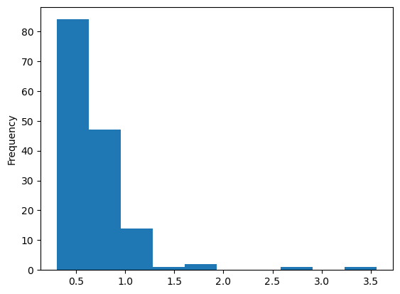
With that, we could start visualizing and analyzing our data via inferential statistics. Regarding the former, pandas even has some built-in functions for basic plotting. Here, some spoilers: a histogram for movie ratings

cleaned_df[cleaned_df['congruent']==1]['resp.rt'].plot.hist()

<Axes: ylabel='Frequency'>

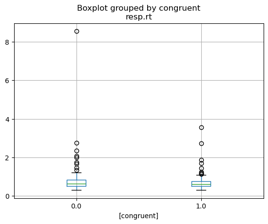
and a boxplot for ratings across categories:

cleaned_df[['congruent', 'resp.rt']].boxplot(by='congruent')

<Axes: title={'center': 'resp.rt'}, xlabel='[congruent]'>

Sorry, but that’s enough spoilers…way more on data visualization next week! For now, we should definitely save the concatenated dataframe as we need it for everything that follows!

cleaned_df.to_csv('data_experiment/preprocessing/cleaned_df_group.csv', index=False)

Outro/Q&A

What we went through in this session was intended as a super small showcase of working with certain data formats and files in python, specifically using pandas which we only just started to explore and has way more functionality.

Sure: this was a very specific use case and data but the steps and underlying principles are transferable to the majority of data handling/wrangling problems/tasks you might encounter. As always: make sure to check the fantastic docs of the python module you’re using (https://pandas.pydata.org/), as well as all the fantastic tutorials out there.

We can explore its functions via pd. and then using tab completion.

pd.

The core Python “data science” stack

• The Python ecosystem contains tens of thousands of packages

• Several are very widely used in data science applications:

  • Jupyter: interactive notebooks

  • Numpy: numerical computing in Python

  • pandas: data structures for Python

  • Scipy: scientific Python tools

  • Matplotlib: plotting in Python

  • scikit-learn: machine learning in Python

• We’ll cover the first three very briefly here

  • Other tutorials will go into greater detail on most of the others

The core “Python for psychology” stack

• The Python ecosystem contains tens of thousands of packages

• Several are very widely used in psychology research:

  • Jupyter: interactive notebooks

  • Numpy: numerical computing in Python

  • pandas: data structures for Python

  • Scipy: scientific Python tools

  • Matplotlib: plotting in Python

  • seaborn: plotting in Python

  • scikit-learn: machine learning in Python

  • statsmodels: statistical analyses in Python

  • pingouin: statistical analyses in Python

  • psychopy: running experiments in Python

  • nilearn: brain imaging analyses in `Python``

  • mne: electrophysiology analyses in Python

• Execept scikit-learn, nilearn and mne, we’ll cover all very briefly in this course

  • there are many free tutorials online that will go into greater detail and also cover the other packages